前言
偶然间看到摸鱼咯大佬在和鲸社区发的帖子 geopandas白化 geopandas对等值线进行白化。以往我是用气象家园中的maskout.py函数进行白化的。但使用maskout.py需要结合meteoinfo对地图文件进行查看,相对来说还是比较麻烦的。在这里就记录一下使用geopandas的方法。
以下用的数据存放在网盘中
百度网盘:j4d3
代码示例
1
2
3
4
5
6
7
8
9
10
11
12
13
14
15
16
import proplot as ppltimport xarray as xrimport pandas as pdimport numpy as npdata = xr.open_dataset('D:/data_english/era5/slp.sst.pre.1979-2020mon.global.nc' ) slp = data['msl' ][:,0 ,...].sel(latitude=slice (None ,None ,4 ), longitude=slice (None ,None ,4 )) lon, lat = np.meshgrid(slp.longitude, slp.latitude) gb = slp.groupby('time.month' ) clim = gb.mean(dim="time" ) slpa = gb - clim slpa = slpa[0 ,...]
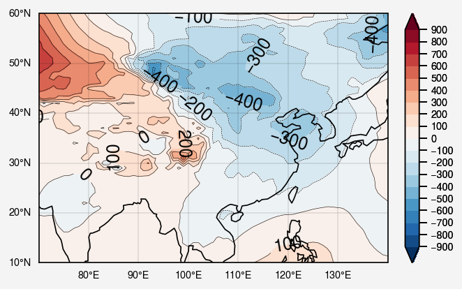
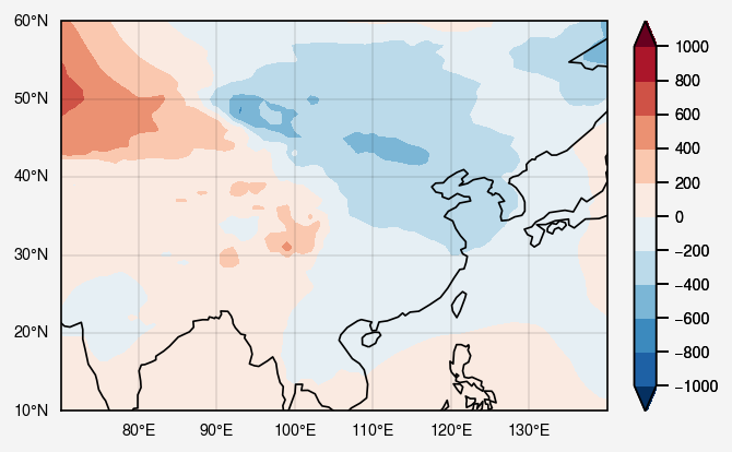
未白化的状况
只看中国周围吧
1
2
3
4
5
6
7
8
9
10
11
12
13
14
15
16
fig, ax = pplt.subplots(proj='cyl' , lonlim=(70 , 140 ), latlim=(10 , 60 )) kw = {'cmap' :'RdBu' , 'extend' :'both' , 'symmetric' :True } fill = ax[0 ].contourf(lon, lat, slpa, **kw, vmin=-900 ) ax.format (labels=True , coast=True , gridlabelsize='xx-small' ) fig.colorbar(fill, label='' , ticklabelsize='xx-small' , width=0.1 )
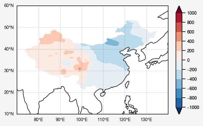
geopandas 读取 shp
下面利用bou2_4p.shp对中国区域进行白化。先看一下geopandas读取shp文件的结果。
1
2
3
4
5
6
7
8
9
import geopandas as gpdfrom shapely.geometry import Pointfrom matplotlib.path import Pathfrom cartopy.mpl.patch import geos_to_pathimport cartopy.crs as ccrsshp = gpd.read_file('bou2_4p.shp' ,encoding='gbk' ) shp
1
2
3
4
5
6
7
8
9
10
11
12
AREA PERIMETER BOU2_4M_ BOU2_4M_ID ADCODE93 ADCODE99 NAME geometry 0 54.447 68.489 2 23 230000 230000 黑龙江省 POLYGON ((121.48844 53.33265, 121.49954 53.336... 1 129.113 129.933 3 15 150000 150000 内蒙古自治区 POLYGON ((121.48844 53.33265, 121.49738 53.321... 2 175.591 84.905 4 65 650000 650000 新疆维吾尔自治区 POLYGON ((96.38329 42.72696, 96.35991 42.70969... 3 21.315 41.186 5 22 220000 220000 吉林省 POLYGON ((123.17104 46.24668, 123.21857 46.269... 4 15.603 38.379 6 21 210000 210000 辽宁省 POLYGON ((123.69019 43.37677, 123.70496 43.381... ... ... ... ... ... ... ... ... ... 920 0.000 0.037 922 3110 810000 810000 香港特别行政区 POLYGON ((114.24527 22.18337, 114.24348 22.184... 921 0.000 0.018 923 3109 810000 810000 香港特别行政区 POLYGON ((114.28620 22.18478, 114.28435 22.185... 922 0.000 0.014 924 3112 810000 810000 香港特别行政区 POLYGON ((114.30350 22.18492, 114.30413 22.186... 923 0.000 0.079 925 3114 810000 810000 香港特别行政区 POLYGON ((114.25628 22.16027, 114.25436 22.163... 924 0.000 0.011 926 3115 810000 810000 香港特别行政区 POLYGON ((114.29893 22.17812, 114.30064 22.178...
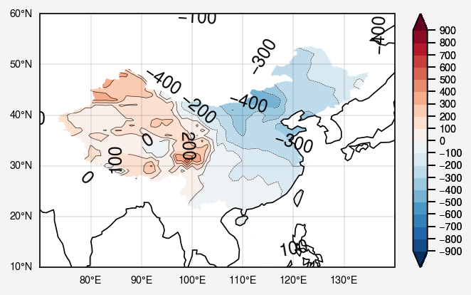
关键白化操作
1
2
3
4
5
6
china = shp['geometry' ].tolist() path_clip = Path.make_compound_path(*geos_to_path(china)) [collection.set_clip_path(path_clip, transform=ax.transData) for collection in fill.collections]
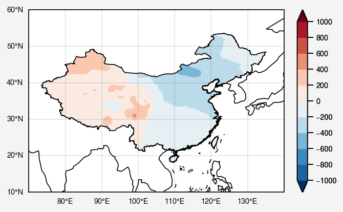
可直接添加图窗画区域边缘
1 2 3 4 5 shp2 = gpd.read_file('bou1_4l.shp' ,encoding='gbk' ) ax.add_geometries(shp2['geometry' ].tolist(), crs=ccrs.PlateCarree(), facecolor='none' , edgecolor='black' ) fig
合并添加多个shp
1 2 3 4 5 6 7 8 9 10 shp = gpd.read_file('bou2_4p.shp' ,encoding='gbk' ) shp2 = gpd.read_file('bou1_4l.shp' ,encoding='gbk' ) com = shp2['geometry' ].append(shp['geometry' ]) ax.add_geometries(com, crs=ccrs.PlateCarree(), facecolor='none' , edgecolor='black' ) fig
风矢量的白化
quiver生成的对象与contourf生成的对象不同,它不包含collection属性。所以白化操作略有不同。
1 2 3 4 5 6 7 8 9 10 11 12 13 14 15 16 17 data2 = xr.open_dataset('GH.UV.500_850hPa.1979-2020.nc' ) u = data2['u' ][:,0 ,0 ,...].sel(latitude=slice (60 ,10 ,4 ), longitude=slice (70 ,140 ,4 )) v = data2['v' ][:,0 ,0 ,...].sel(latitude=slice (60 ,10 ,4 ), longitude=slice (70 ,140 ,4 )) gb = u.groupby('time.month' ) clim = gb.mean(dim="time" ) ua = gb - clim ua = ua[0 ,...] gb = v.groupby('time.month' ) clim = gb.mean(dim="time" ) va = gb - clim va = va[0 ,...] lon2, lat2 = np.meshgrid(u.longitude,v.latitude)
1 2 3 4 5 d=1 tt = ax.quiver(lon2[::d,::d],lat2[::d,::d],ua[::d,::d],va[::d,::d]) tt.set_clip_path(path_clip, transform=ax.transData)
对于quiver,数据范围最好保证在extent范围内。如果使用-180~180的数据,而extent只设定在70-120,那么画出来的矢量箭头会非常小,需要手动调整scale。一般来说需要进一步调整降低箭头密集度,并调整scale
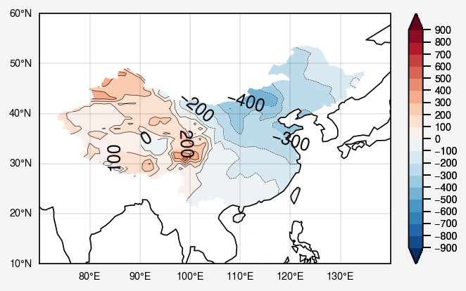
contour 和 clabel的白化
contour的白化方法与contourf白化方法相同。contour生成对象后,提取collection循环切片即可。
1 2 3 4 5 6 7 8 9 10 11 12 13 14 15 16 17 18 19 20 21 22 23 import proplot as ppltimport xarray as xrimport pandas as pdimport numpy as npimport geopandas as gpdfrom matplotlib.path import Pathfrom cartopy.mpl.patch import geos_to_pathimport cartopy.crs as ccrsfrom shapely.geometry import Polygon as ShapelyPolygonfrom shapely.geometry import Point as ShapelyPointdata = xr.open_dataset('D:/data_english/era5/slp.sst.pre.1979-2020mon.global.nc' ) slp = data['msl' ][:,0 ,...].sel(latitude=slice (None ,None ,4 ), longitude=slice (None ,None ,4 )) lon, lat = np.meshgrid(slp.longitude, slp.latitude) gb = slp.groupby('time.month' ) clim = gb.mean(dim="time" ) slpa = gb - clim slpa = slpa[0 ,...]
1 2 3 4 5 6 7 8 9 10 11 12 13 fig, ax = pplt.subplots(proj='cyl' ,lonlim=(70 , 140 ), latlim=(10 , 60 )) kw = { 'cmap' :'RdBu_r' ,'extend' :'both' , 'symmetric' :True } fill = ax[0 ].contourf(lon, lat, slpa, **kw, vmin=-900 ,values=20 ) con = ax[0 ].contour(lon, lat, slpa, levels=fill.levels, color='black' ,linewidth=0.2 ) cb = ax[0 ].clabel(con,levels=fill.levels) ax.format (labels=True , coast=True , gridlabelsize='xx-small' ) fig.colorbar(fill, label='' , ticklabelsize='xx-small' , width=0.1 )
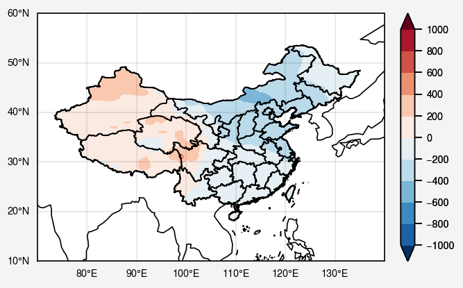
下面对等值线白化
1
2
3
4
5
6
7
8
9
10
11
12
13
14
15
16
shp = gpd.read_file('D:/anaconda_spyder_filesave/mission/mission9/0619/shpfile/bou2_4p.shp' ,encoding='gbk' ) ee = shp['geometry' ].tolist() path_clip = Path.make_compound_path(*geos_to_path(ee)) [collection.set_clip_path(path_clip, transform=ax.transData) for collection in fill.collections] [collection.set_clip_path(path_clip, transform=ax.transData) for collection in con.collections] fig
可以看到labels还是到处乱飞,下面需要对labels白化。然而labels对象是Text组成的列表,操作过程以上等值线白化又有不同。
1 2 3 4 5 6 7 for text_object in cb: if not path_clip.contains_point(text_object.get_position()): text_object.set_visible(False ) fig
path_clip.contains_point 判断点是否在路径所包围的区域内
非等经纬度投影白化
以上白化操作ax的投影皆为ccrs.PlateCarree(), 数据投影也为ccrs.PlateCarree()。因此无论是画图还是白化都不需要额外的操作来转化点的坐标。
需要注意的是,在创建ax时,projection参数是对ax进行投影设置。即若projection=ccrs.PlateCarree(),则我们最后看到的图就是等经纬度投影的图。若projection=ccrs.LambertConformal(),则我们最后看到的图就是兰伯特投影的样子。
然而在contourf的transform和ax.set_extent()中设置的crs的意义不同,它们要求我们告诉程序,为什么所输入的数据是取自怎样的投影。一般来说,我们的数据都是格点数据,lon:-180~180, lat:-90~90。即我们的数据一般是等经纬度的,所以transform和crs都设置为ccrs.PlateCarree()就可以了(不随projection的变化而变化)。
详情可以看这里 transform和projection的意义
此外,通常我们的shp文件提取出的点也是等经纬度的lon:-180~180, lat:-90~90。而当projection=ccrs.LambertConformal()时就无法直接用以上程序直接进行白化,因为坐标不对应。这个时候需要先将路径Path转化到相应的projection上。
注意即使我们的projection使用的是ccrs.PlateCarree(),但设置了中心经度例如projection=ccrs.PlateCarree(central_longitude=120)。也需要对路径点进行坐标转化。路径点坐标系必须与 projection 完全一致
1 2 3 4 5 6 7 8 9 10 11 12 13 14 15 path_clip = Path.make_compound_path(*geos_to_path(ee)) codes = path_clip.codes pp = ccrs.LambertConformal(central_longitude=100 , central_latitude=30 ) path_clip = Path(pp.transform_points(ccrs.PlateCarree(),path_clip.vertices[:,0 ], path_clip.vertices[:,1 ])[:,0 :2 ],codes=codes)
codes似乎标记了多边形个体,每个多边形用有一个数字存在codes中。如果不添加codes参数,例如大陆和海南岛之间会有路径穿过。
摸鱼咯大佬的帖子中使用的是ccrs.Geodetic()而不是ccrs.PlateCarree()来转化路径点,我不清楚有什么区别。我觉得ccrs.PlateCarree()更合理一些。
由此,我们得到了一个新的path_clip,后面的白化过程就与之前的内容完全一致了。如果我们不是用等经纬度投影创建坐标轴,就需要将路径点的坐标转化到相应的projection上。
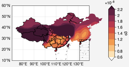
南海小图
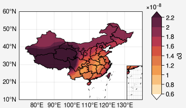
有时候在画中国地图时需要对地图右下角添加一个小图来显示南海地区。这个小图可以和主图完全相同,只需要调整extent即可。然而,在白化之后会出现如下图的情况。
小图范围内虽然白化成功,但是小图之外的图像并没有去除掉。原因在于ax.set_extent()和collection.set_clip()这两个命令相互覆盖了。导致只有一个命令生效。解决的方法就是找到extent与path_clip的交集。思路来源于:链接
1
2
3
4
5
6
7
8
9
10
11
12
13
14
15
16
17
18
19
20
21
22
23
24
25
26
27
28
29
30
from shapely import geometry as geofrom cartopy.mpl.patch import geos_to_path,path_to_geosiax = ax.inset([140 -11 *0.8 ,10 ,11 *0.8 ,24 *0.8 ],transform='data' ) fill2 = iax.contourf(lon, lat, o3, extend='both' , robust=True ) iax.add_geometries(shp['geometry' ], crs=ccrs.PlateCarree(), facecolor='None' , ) iax.add_geometries(shp2['geometry' ], crs=ccrs.PlateCarree(), facecolor='None' , ) iax.format (lonlim=(109 ,120 ), latlim=(0 ,24 )) extent = [109 ,120 ,0 ,24 ] extentPolygon = geo.Polygon([ (extent[0 ], extent[2 ]), (extent[0 ], extent[3 ]), (extent[1 ], extent[3 ]), (extent[1 ], extent[2 ]), (extent[0 ], extent[2 ]), ]) polygon_clip = [] for p in path_to_geos(path_clip): polygon_clip.append(extentPolygon.intersection(p)) path_clip2 = Path.make_compound_path(*geos_to_path(polygon_clip)) [collection.set_clip_path(path_clip2, transform=iax.transData) for collection in fill2.collections]
总结
写了这么多,再回去看看觉得好乱。那就简单做个总结吧。
文件读取
1
2
3
4
import geopandas as gpdshp = gpd.read_file('./shpfile/china.shp' ) china = shp['geometry' ].tolist()
剪切路径
1
2
3
4
5
6
7
8
9
10
11
from matplotlib.path import Pathfrom cartopy.mpl.patch import geos_to_pathimport cartopy.crs as ccrspath_clip = Path.make_compound_path(*geos_to_path(china)) codes = path_clip.codes pp = ccrs.LambertConformal(central_longitude=100 , central_latitude=30 ) path_clip = Path(pp.transform_points(ccrs.PlateCarree(),path_clip.vertices[:,0 ], path_clip.vertices[:,1 ])[:,0 :2 ],codes=codes)
等值线和填色图白化
1 2 3 4 [collection.set_clip_path(path_clip, transform=ax.transData) for collection in fill.collections] [collection.set_clip_path(path_clip, transform=ax.transData) for collection in con.collections]
风矢量白化
1 2 tt.set_clip_path(path_clip, transform=ax.transData)
clabel 白化
1 2 3 4 for text_object in cb: if not path_clip.contains_point(text_object.get_position()): text_object.set_visible(False )
polygon取交集白化
1 2 3 4 5 6 7 8 polygon_clip = [] for p in path_to_geos(path_clip): polygon_clip.append(extentPolygon.intersection(p)) path_clip2 = Path.make_compound_path(*geos_to_path(polygon_clip)) [collection.set_clip_path(path_clip2, transform=iax.transData) for collection in fill2.collections]

 对于quiver,数据范围最好保证在extent范围内。如果使用-180~180的数据,而extent只设定在70-120,那么画出来的矢量箭头会非常小,需要手动调整scale。一般来说需要进一步调整降低箭头密集度,并调整scale